Müller's Method

yet another iterative root finding algorithm. Combination of Regula Falsi and Newton-Raphson

1. The Core Idea: Parabola, not a Line

• Regula Falsi (False Position) approximates the function $f(x)$ by drawing a line (a 1st-degree polynomial) through two points, $(a,f(a))$ and $(b,f(b))$.

• Newton-Raphson approximates the function $f(x)$ by drawing a tangent line (also a 1st-degree polynomial) at one point, $(x_n,f(x_n))$, using the derivative.

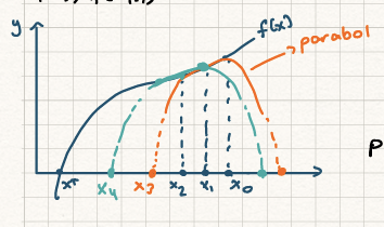
• Müller’s Method takes this one step further. It approximates the function $f(x)$ by drawing a parabola (a 2nd-degree polynomial, $p(x)=a{x}^2+bx+c$) that passes through three initial points: $(x_0,f(x_0))$, $(x_1,f(x_1))$, and $(x_2,f(x_2))$.

So,

• We start with three guesses: $x_0$, $x_1$, and $x_2$.

• We draw a unique parabola $p(x)$ (the blue curve) that perfectly intersects $f(x)$ (the orange curve) at all three of these points.

  g(x0) = f(x0) and such.

• A parabola can intersect the x-axis at zero, one, or two points. We find these intersections.

• Our new guess, $x_3$, is the intersection that is closest to our last guess ($x_2$).

• To find the next guess ($x_4$), we would “forget” the oldest point ($x_0$) and repeat the process using the points $(x_1,x_2,x_3)$.

The mathematics

The goal is to find the roots of the parabola $p(x)$ as our new approximation.

Step 1: Define the Parabola in a Clever Way

Instead of the standard $p(x)=a{x}^2+bx+c$, the notes use a form centered around the most recent point, $x_i$ (in the graph’s first step, this would be $x_2$). This is Newton’s form of an interpolating polynomial:

$p_i(x)=a_i(x-x_i{)}^2+b_i(x-x_i)+c_i$

This form is much easier to work with. We find the coefficients $a_i,b_i,c_i$ by forcing the parabola to pass through our three known points:

• $p_i(x_i)=f(x_i)$

• $p_i(x_{i-1})=f(x_{i-1})$

• $p_i(x_{i-2})=f(x_{i-2})$

Plugging $x=x_i$ into the equation is very simple:

$p_i(x_i)=a_i(x_i-x_i{)}^2+b_i(x_i-x_i)+c_i=c_i$.

So, we instantly find $c_i=f(x_i)$.

We can then use the other two points to create a 2x2 system of equations to find $a_i$ and $b_i$. The notes skip this algebra and just state, “Now we know $a_i,b_i,c_i$ coefficients.”

Step 2: Find the Zeros of the Parabola

We need to solve $p_i(x)=0$ for our next guess, $x_{i+1}$.

$a_i(x_{i+1}-x_i{)}^2+b_i(x_{i+1}-x_i)+c_i=0$

This is just a quadratic equation for the step size $z=(x_{i+1}-x_i)$. Using the standard quadratic formula $z=\frac{-b\pm \sqrt{b^2-4ac}}{2a}$, we get:

$x_{i+1}-x_i=\frac{-b_i\pm \sqrt{b_i^2-4a_i{c}_i}}{2a_i}$

Step 3: A More Numerically Stable Formula

The standard quadratic formula can be bad for computers. If $b_i^2$ is very large compared to $4a_i{c}_i$, then $\sqrt{b_i^2-4a_i{c}_i}\approx \sqrt{b_i^2}\approx |b_i|$. This means the numerator might become $-b_i+b_i=0$, a problem called catastrophic cancellation that destroys precision.

To fix this, the notes use a common trick: multiply the numerator and denominator by the conjugate (as noted by “eşlenik ile çarp”):

$x_{i+1}-x_i=\left[\frac{-b_i\pm \sqrt{b_i^2-4a_i{c}_i}}{2a_i}\right]\cdot \left[\frac{-b_i\mp \sqrt{b_i^2-4a_i{c}_i}}{-b_i\mp \sqrt{b_i^2-4a_i{c}_i}}\right]$

• The numerator becomes: $(-b_i{)}^2-(\sqrt{b_i^2-4a_i{c}_i}{)}^2=b_i^2-(b_i^2-4a_i{c}_i)=4a_i{c}_i$

• The denominator becomes: $2a_i(-b_i\mp \sqrt{b_i^2-4a_i{c}_i})$

Canceling the $2a_i$ term gives the new, more stable formula shown on the slide:

$x_{i+1}-x_i=\frac{2c_i}{-b_i\mp \sqrt{b_i^2-4a_i{c}_i}}$

This formula has “two possibilities” (the $\mp$). The * note explains how to choose:

• We pick the sign in the denominator ($\mp$) to be the same as the sign of $b_i$. For example, if $b_i$ is positive, we use $-b_i-\sqrt{\dots }$.

• This forces the two terms in the denominator to add together, making the denominator’s magnitude as large as possible.

• A larger denominator gives a smaller step size $(x_{i+1}-x_i)$, which corresponds to the root of the parabola that is closest to our current guess $x_i$.

3. Convergence

The final note, “The order of convergence is $\approx 1.839$ (konu dışı - off-topic),” is a key takeaway.

• Regula Falsi is linear ($p=1$).

• Newton-Raphson is quadratic ($p=2$).

• Müller’s Method is superlinear ($p\approx 1.839$).

It is significantly faster than linear methods and, while not as fast as Newton’s method, it has a major advantage: you do not need to calculate the derivative $f^{\prime }(x)$, which can be difficult or impossible for some functions.